Mathematical Background ¶

The software package ttrr emerged from the scientific research for [Mohr2011], [MohrSteinMatziesKnapek2012] and [MohrSteinMatziesKnapek2013].

First, I started with MatLab http://www.mathworks.de/ in my PhD research, but the problems were too hard for this great software package. Furthermore, MatLab does not support the solving of mixed integer programs on its own. Therefore I was looking for something else: I found GLPK http://www.gnu.org/software/glpk/ and Python http://www.python.org/ — both are great software!

Because it was simple, I did the visualization with MatLab http://www.mathworks.de/ in my PhD-thesis [Mohr2011]. To write ttrr, I do not want to use a commercial back end for the visualization or moreover point you to such a software. But if you like, you can do it on your own.

Contents

Mathematical Background

General Concept of Topology Optimization of Truss ¶

Truss topology optimization has its root in [Michell1904].

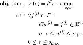
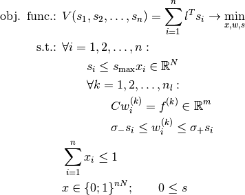
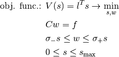
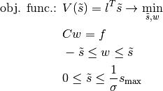
The analytically stated and known (cf. [Przemieniecki1968]; [Marti2003]; [BendsoeSigmund2004]) linear problem of the topology optimization of a truss with respect to its volume (plastic design) is given by the objective function to be minimized

$\begin{align*} \min_{s,w}{l^T s} \end{align*}$

with the bar lengths $l \in \R^n$ subject to the equilibrium condition

$\begin{align*} C w = f \end{align*}$

with the reduced geometry matrix $C \in \R^{m \times n}$ , the inner bar forces $w \in \R^n$ and the reduced applied external loads $f \in \R^m$ . Further given are the constraints

$\begin{align*} \sigma_- s \leq w \leq \sigma_+ s \end{align*}$

for the linear elasticity by — for all bars equal — stress limits $0 > \sigma_- \in \R$ and $0 < \sigma_+ \in \R$ (e. g. yield points for pressure and tension of the material all bars are made of), and the box constraint

$\begin{align*} 0 \leq s \leq s_{\max} \end{align*}$

for the cross sections of the bars $s \in \R^n$ with the given maximal bar cross section $s_{\max} \in \R^n$ . [1]

Here $w$ is seen as a design variable; otherwise we have $s(w)$ as function and therefore no linear program.

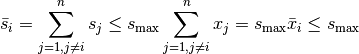
If more than one load (e. g. the set $F$ of loads) is to be considered, one ends up at the known multiple load case. But how is it performed? How can we put more than one load in the above linear program? It is impossible! But we can ask for a robust solution — this means we consider the worst case: A solution for all $f^{(i)} \in F$ is searched. Now we really end up at the well known multiple load case: [3]

$\begin{align*} \mbox{obj. func.: }&V(s) = l^T s \rightarrow \min_{s,w} \\ \mbox{s.t.: } & \forall f^{(i)} \in F: & \\ & \qquad C w^{(i)} = f^{(i)} \in \R^m \\ & \qquad \sigma_- s \leq w^{(i)} \leq \sigma_+ s \\ & 0 \leq s \leq s_{\max} \end{align*}$

All this is done by ttrr.ttrr().

[1]	The maximal cross section is no limitation — it’s a feature! It provides the possibility to limit the cross section; but if you do not want this set a huge upper limit — but an adequate limit helps the optimization algorithms.

[3]	Sorry for the compactness, but you can look at the literature all over the world. :-)

Robust Topology Optimization of Truss ¶

For robust optimization see [Ben-TalElGhaouiNemirovski2009].

The implementation in ttrr.ttrr_robust() follows [MohrSteinMatziesKnapek2012]. This means if perturbed loads $\tilde{F}$ are given, they are composed by some perturbations of the unperturbed force $f$ . Due to the linear programming we can restrict ourselves to the extreme points of $\tilde{F}$ .

If we start the other way round with an additional assumption, it becomes clear: Let $f$ be a given force with a perturbation of $10 \mbox{\%}$ . Then we are interested in a solution for all 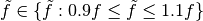$\tilde{f} \in \{\tilde{f} : 0.9 f \leq \tilde{f} \leq 1.1 f\}$ . Obviously the extreme points are $0.9 f$ and $1.1 f$ . Therefore a solution for all loads in the set $F := \{0.9 f ; 1.1 f\}$ is searched.

So robust optimization in topology optimization is the same as the multiple load case with appropriate load cases. For $F$ a polyhedron a finite number of extreme points is given. And therefore ttrr.ttrr() can be recycled.

In addition ttrr.ttrr_robust() provides features to calculate the extreme points of simple sets of perturbed forces.

Redundant Topology Optimization of Truss ¶

The basic concept of topology optimization with regard to redundancy is described in [Mohr2011] and in [MohrSteinMatziesKnapek2013].

Redundant Topology Optimization of Truss means we are looking for the best topology of a truss with a redundancy as to the falling out of some parts of the structure. The dream is a structure which is functional even if a significant damage occurs to an arbitrary set of bars.

You should think of RAID [4]. [PattersonGibsonKatz1987]

For example, a RAID 1 is a bunch of discs and every disc does the work. This means every other one can fail. Following [Mohr2011] this is called “1-1/n”-redundancy (c.f. [Shannon1948] [PattersonGibsonKatz1987]). Transferred to structures this means we are looking for $n$ different structures in the same design space fulfilling the task to sustain the load(s).

Let $s_i \in \R^N$ be the cross sections of the bars for the structure $i$ . The sum $s = \sum_{i=1}^{n}{s_i}$ describes the cross sections of the bars for the complete structure. The complete structure is composed of the $n$ structures $s_i$ . With the selecting variables $x_i \in \{0;1\}^N$ we can now formulate the problem as a mixed integer linear program: [5]

$\begin{align*} \mbox{obj. func.: }&V(s_1,s_2,\ldots,s_n) = \sum_{i=1}^{n}{l^T s_i} \rightarrow \min_{x,w,s} \\ \mbox{s.t.: } & \forall i=1,2,\ldots,n: \\ & \qquad s_i \leq s_{\max} x_i \in \R^N \\ & \qquad \forall k=1,2,\ldots,n_l: \\ & \qquad \qquad C w_i^{(k)} = f^{(k)} \in \R^m \\ & \qquad \qquad \sigma_- s_i \leq w_i^{(k)} \leq \sigma_+ s_i \\ & \sum_{i=1}^{n}{x_i} \leq 1 \\ & x \in \{0;1\}^{nN} ; \qquad 0 \leq s \end{align*}$

From $x \in \{0;1\}^{nN}$ follows $0 \leq \sum_{i=1}^{n}{x_i}$ and $s \leq s_{\max}$ .

This is done by ttrr.ttrr_redundant() for redundancy = $-n \leq -2$ .

A RAID 5 (c.f. [PattersonGibsonKatz1987]) is more complex. It can be described as a simple code. To transfer this concept to structures we only need to know the behavior. A RAID 5 is a bunch of discs. Every single disc may fail and the others do the job together. Following [Mohr2011] this is called “1/n”-redundancy (c.f. [Shannon1948] [PattersonGibsonKatz1987]). Back to structures this means we are looking for $n$ different structures in the same design space. Every single structure can fall out and the other ones should sustain the load(s) together.

Let $s_i \in \R^N$ be the cross sections of the bars for the structure $i$ . As before $s = \sum_{i=1}^{n}{s_i}$ describes the cross sections of the bars for the complete structure. The complete structure $s$ is composed of the $n$ structures $s_i$ . If a structure $i$ fall out, the resulting structure is 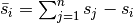$\bar{s}_i = \sum_{j=1}^{n}{s_j} - s_i$ . As mentioned before, this damaged structure should sustain the load(s).

With the selecting variables $x_i \in \{0;1\}^N$ we can now formulate the problem as a mixed integer linear program: [5]

$\begin{align*} \mbox{obj. func.: }&V(s_1,s_2,\ldots,s_n) = \sum_{i=1}^{n}{l^T s_i} \rightarrow \min_{x,w,s} \\ \mbox{s.t.: } & \forall i=1,2,\ldots,n: \\ & \qquad s_i \leq s_{\max} x_i \in \R^N \\ & \qquad \forall k=1,2,\ldots,n_l: \\ & \qquad \qquad C w_i^{(k)} = f^{(k)} \in \R^m \\ & \qquad \qquad \sigma_- \bar{s}_i \leq w_i^{(k)} \leq \sigma_+ \bar{s}_i \\ & \sum_{i=1}^{n}{x_i} \leq 1 \\ & x \in \{0;1\}^{nN} ; \qquad 0 \leq s \\ \mbox{with: } & \bar{x}_i = \sum_{j=1, j \ne i}^{n}{x_j} ; \qquad \bar{s}_i = \sum_{j=1, j \ne i}^{n}{s_j} \end{align*}$

Trivially $0 \leq \sum_{i=1}^{n}{\bar{x}_i} \leq 1$ holds and therefore $0 \leq \bar{x}_i \leq 1$ . From $x \in \{0;1\}^{nN}$ follows $0 \leq \sum_{i=1}^{n}{x_i}$ and $s \leq s_{\max}$ . The damaged structures are also well defined:

$\bar{s}_i = \sum_{j=1, j \ne i}^{n}{s_j} \leq s_{\max} \sum_{j=1, j \ne i}^{n}{x_j} = s_{\max} \bar{x}_i \leq s_{\max}$

Clearly $0 \leq \bar{s}_i$ holds. So we get for the damaged structures 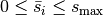$0 \leq \bar{s}_i \leq s_{\max}$ and for the complete structure $0 \leq s \leq s_{\max}$ .

This is done by ttrr.ttrr_redundant() for redundancy = $n \geq 2$ .

[4]	RAID is an acronym for Redundant Array of Independent Disks. http://en.wikipedia.org/wiki/RAID

[5]	(1, 2) MIP: mixed integer problem; MILP: mixed integer linear program. Because MIP in general is too time consuming everybody is only thinking of MILP and often calls it MIP.

Robust Redundant Topology Optimization of Truss ¶

Robust redundant topology optimization is nothing more than redundant topology optimization with appropriate load cases. This concept of redundant robust topology optimization is described in [MohrSteinMatziesKnapek2013].

$digraph succession { rankdir=LR; "robust" [label="ttrr.ttrr_robust"]; "perturbaton" [label="if necessary:\ncreate perturbed forces"]; "ttrr" [label="ttrr.ttrr"]; "redundant" [label="ttrr.ttrr_redundant"]; "robust" -> "perturbaton" -> "ttrr"; "perturbaton" -> "redundant"; }$

Uniqueness of the solution ¶

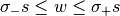
For a linear problem possibly more than one edge of the polyhedron exists as a solution. So the solution of a linear problem is not unique — but the optimal object value is.

Let us consider the small example:

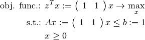
$\begin{align*} \mbox{obj. func.: }& z^T x := \left(\begin{array}{cc}1&1\\\end{array}\right) x \rightarrow \max_{x} \\ \mbox{s.t.: } & A x := \left(\begin{array}{cc}1&1\\\end{array}\right) x \leq b := 1 \\ & x \geq 0 \end{align*}$

A visualization is given in Fig. Visualization of the simple LP.

Visualization of the simple LP

In the visualization we see a level curve for $z^T x = 0$ and the polyhedron $\{x \in \R^2 : A x \leq b \wedge x \geq 0\}$ bounded by the constraints.

Without a lengthy calculation we can see that the optimal value of the objective function $z^T x$ is $1$ . The edges $(0,1)$ and $(1,0)$ are feasible, optimal and have both the same value of the objective function — the same for all points between these edges.

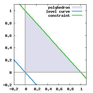
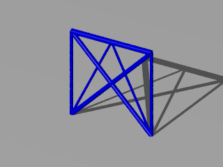
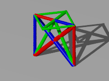
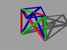
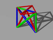
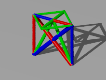
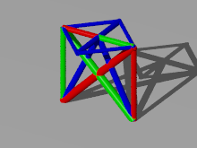
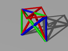
So in general you cannot expect a unique solution for a linear program. The simplex algorithm will find an edge as a solution. An interior point algorithm will typically find a solution between edges which are optimal. The following two pictures from Example: 2_load_cases_3_dim show this behavior — both are optimal for the same problem.

simplex interior point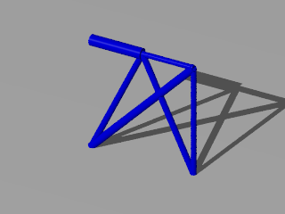

For the redundant topology optimization we have in every case more than one solution. For example let $\tilde{x},\tilde{w},\tilde{s}$ with $\tilde{s} = (\tilde{s}_1,\tilde{s}_2,\ldots,\tilde{s}_n)$ be a solution, then $(\tilde{s}_2,\tilde{s}_1,\ldots,\tilde{s}_n)$ is one, too.

For the example Example: 2_load_cases_3_dim for a “1/3”-redundancy this is shown in the following table:

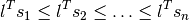
To mostly overcome this behavior we can require an order of the volumes of the structures:

$l^T s_1 \leq l^T s_2 \leq \ldots \leq l^T s_n$

This is implemented in ttrr.ttrr_redundant() with the flag “sort”.

Scaling Factors ¶

To look at scaling behavior of the above linear programs let us consider the following structure:

$\begin{align*} \mbox{obj. func.: }&V(s) = l^T s \rightarrow \min_{s,w} \\ & C w = f \\ & \sigma_- s \leq w \leq \sigma_+ s \\ & 0 \leq s \leq s_{\max} \end{align*}$

Material, Load and Design Space ¶

The material parameters for the topology optimization of truss given to ttrr.ttrr(), ttrr.ttrr_robust() or ttrr.ttrr_redundant() are:

$s_{\max}$ : the maximal allowed cross section of a bar

$\sigma_-$ : lower limit for the allowed stress, e.g. compressive strength

$\sigma_+$ : upper limit for the allowed stress, e.g. tensile strength

density : density

The density is only used to calculate the mass of the structure out of its volume.

$s_{\max}$ is necessary for ttrr.ttrr_redundant() and gives an additional feature to ttrr.ttrr() and ttrr.ttrr_robust(). If its not wanted a huge value would disable it. But in any case it gives with $0 \leq s \leq s_{\max}$ bounding values. So we have a closed feasible region.

$\sigma_-$ and $\sigma_+$ are really used material parameters. Typical topology optimization is a preliminary design. Therefore it must not be totally accurate to the praxis. Typically 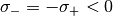$\sigma_- = -\sigma_+ < 0$ is chosen. So we can assume $\sigma_- = -\sigma_+ = -\sigma$ for some $\sigma > 0$ .

$\begin{align*} \mbox{obj. func.: }&V(s) = l^T s \rightarrow \min_{s,w} \\ & C w = f \\ & -\sigma s \leq w \leq \sigma s \\ & 0 \leq s \leq s_{\max} \end{align*}$

Easily to see the following program results in an equivalent optimum. With $\tilde{s} = \sigma s$ we get:

$\begin{align*} \mbox{obj. func.: }&V(\tilde{s}) = l^T \tilde{s} \rightarrow \min_{\tilde{s},w} \\ & C w = f \\ & -\tilde{s} \leq w \leq \tilde{s} \\ & 0 \leq \tilde{s} \leq \frac{1}{\sigma} s_{\max} \end{align*}$

This is only a scaling. The magnitude of the loads is only a scaling, too. With $\tilde{w} = \alpha w$ for some $\alpha > 0$ we get:

$\begin{align*} \mbox{obj. func.: }&V(\tilde{s}) = l^T \tilde{s} \rightarrow \min_{\tilde{s},\tilde{w}} \\ & C \tilde{w} = \alpha f \\ & -\alpha \tilde{s} \leq \tilde{w} \leq \alpha \tilde{s} \\ & 0 \leq \tilde{s} \leq \frac{1}{\sigma} s_{\max} \end{align*}$

And furthermore with 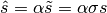$\hat{s} = \alpha \tilde{s} = \alpha \sigma s$ the following program is equivalent, too:

$\begin{align*} \mbox{obj. func.: }&V(\hat{s}) = l^T \hat{s} \rightarrow \min_{\hat{s},\tilde{w}} \\ & C \tilde{w} = \alpha f \\ & - \hat{s} \leq \tilde{w} \leq \alpha \hat{s} \\ & 0 \leq \hat{s} \leq \frac{1}{\alpha \sigma} s_{\max} \end{align*}$

Keep in mind it is not required to change the objective function. For $\beta > 0$ the minimum of the functions $g(x)$ and $\beta g(x)$ is reached at the same point.

The size of the design space is not found directly in the linear program. In the geometry matrix $C$ occur only the angles of the bars. So the magnitude of the size of the design space in meter or millimeter will result in the same optimal structure, because $l$ is only in the objective function and will be changed by a scalar factor.

Numeric ¶

A scaling of

$\begin{align*} \mbox{obj. func.: }&V(s) = l^T s \rightarrow \min_{s,w} \\ & C w = f \\ & \sigma_- s \leq w \leq \sigma_+ s \\ & 0 \leq s \leq s_{\max} \end{align*}$

do not change the (relative) condition of the problem. But it can change the absolute condition and therefore helps the computer by the calculation.

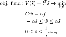
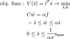
To do so the functions ttrr.ttrr(), ttrr.ttrr_robust() or ttrr.ttrr_redundant() have the parameters $\alpha =$ scale_sigma and $\beta =$ scale_forces. To get the picture let us see how they transform the above problem:

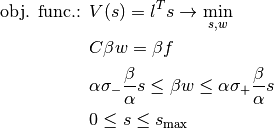
$\begin{align*} \mbox{obj. func.: }&V(s) = l^T s \rightarrow \min_{s,w} \\ & C \beta w = \beta f \\ & \alpha \sigma_- \frac{\beta}{\alpha} s \leq \beta w \leq \alpha \sigma_+ \frac{\beta}{\alpha} s \\ & 0 \leq s \leq s_{\max} \end{align*}$

Now the calculation will be done with $\tilde{s} = \frac{\beta}{\alpha} s$ , $\tilde{w} = \beta w$ , $\tilde{f} = \beta f$ , $\tilde{\sigma}_- = \alpha \sigma_-$ , $\tilde{\sigma}_+ = \alpha \sigma_+$ and $\tilde{s}_{\max} = \frac{\beta}{\alpha} s_{\max}$ :

$\begin{align*} \mbox{obj. func.: }&V(\tilde{s}) = l^T \tilde{s} \rightarrow \min_{\tilde{s},\tilde{w}} \\ & C \tilde{w} = \tilde{f} \\ & \tilde{\sigma}_- \tilde{s} \leq \tilde{w} \leq \tilde{\sigma}_+ \tilde{s} \\ & 0 \leq \tilde{s} \leq \tilde{s}_{\max} \end{align*}$

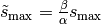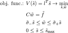
Afterwards $\tilde{s}$ and $\tilde{w}$ will be transformed back.

For a maximum magnitude of $1$ of an element from $\tilde{f}$ the absolute condition of the equation will be a little bit better. For a maximum magnitude of $1$ of an element from $\tilde{\sigma}_-$ and from $\tilde{\sigma}_+$ the condition of the inequation will be significant better. If $\alpha = \beta$ the design variables $s$ and $s_{\max}$ resp. will not be changed.

References:

[Ben-TalElGhaouiNemirovski2009]

Aharon Ben-Tal ; Laurent El Ghaoui ; Arkadi Nemirovski: Robust Optimization. Princeton University Press, 2009. http://press.princeton.edu/titles/9099.html

[BendsoeSigmund2004]

Bendsoe, Martin P. ; Sigmund, Ole: Topology Optimization. Berlin, Heidelberg : Springer, 2004. ISBN 3-540-42992-1

[Marti2003]

Kurt Marti: Stochastic optimization methods in optimal engineering design under stochastic uncertainty. In: ZAMM, 83 (12): 795–811, 2003. http://dx.doi.org/10.1002/zamm.200310072

[Michell1904]

Michell, Anthony George M.: The limits of economy of material in frame structures. In: Phil. Mag. 8 (1904), Nr. 47, S. 589-597. http://dx.doi.org/10.1080/14786440409463229.

[Mohr2011]

(1, 2, 3, 4, 5) Mohr, Daniel P.: Redundante Topologieoptimierung. Neubiberg, Universitaet der Bundeswehr Muenchen, Fakultaet fuer Luft- und Raumfahrttechnik, Diss., Dezember 2011. http://nbn-resolving.de/urn/resolver.pl?urn=urn:nbn:de:bvb:706-2664

[MohrSteinMatziesKnapek2012]

(1, 2) Mohr, Daniel P. ; Stein, Ina ; Matzies, Thomas ; Knapek, Christina A.: Robust Topology Optimization of Truss with regard to Volume. In: arXiv - Mathematics, Optimization and Control (2012). http://arxiv.org/abs/1109.3782v2

[MohrSteinMatziesKnapek2013]

(1, 2, 3) Mohr, Daniel P. ; Stein, Ina ; Matzies, Thomas ; Knapek, Christina A.: Redundant robust topology optimization of truss. In: Optimization and Engineering (2013), 1-28. http://dx.doi.org/10.1007/s11081-013-9241-7

[PattersonGibsonKatz1987]

(1, 2, 3, 4) Patterson, David A. ; Gibson, Garth A. ; Katz, Randy H.: A Case for Redundant Arrays of Inexpensive Disks (RAID). Version: Dec 1987. 1987 (UCB/CSD-87-391). — Forschungsbericht. — EECS Department, University of California, Berkeley. http://www.eecs.berkeley.edu/Pubs/TechRpts/1987/5853.html

[Przemieniecki1968]

Janusz S. Przemieniecki: Theory of matrix structural analysis. McGraw-Hill, Inc., New York, 1968.

[Shannon1948]

(1, 2) Shannon, Claude E.: A Mathematical Theory of Communication. Version: 1948. 1948 (1). — Forschungsbericht. — 379-423, 623-656 S. — The Bell System Technical Journal. http://cm.bell-labs.com/cm/ms/what/shannonday/paper.html

Mathematical Background ¶

General Concept of Topology Optimization of Truss ¶

Robust Topology Optimization of Truss ¶

Redundant Topology Optimization of Truss ¶

Robust Redundant Topology Optimization of Truss ¶

Uniqueness of the solution ¶

Scaling Factors ¶

Material, Load and Design Space ¶

Numeric ¶

Table Of Contents

Previous topic

Next topic

This Page

Navigation

Previous topic

Next topic

This Page

Quick search

Navigation