Example: 2_load_cases_3_dim
Contents
This is a 3 dimensional example to show ttrr.
This example is also available as batch_2_load_cases_3_dim.py.
First start python and import necessary modules:
>>> import ttrr,numpy,scipy
design space
To define the design space:
>>> dim = 3 # dimension of the design space
>>> nelx = 3 # number of nodal points in x-direction
>>> nely = nelx # number of nodal points in y-direction
>>> nelz = nelx # number of nodal points in z-direction
To let you easily change the design space, we use here a calculation to define the grid. The measurement unit is meter:
>>> n = max(nelx,nely,nelz)
>>> gx0 = 0.0
>>> gx1 = (nelx-1)*1.0/(n-1)
>>> gy0 = 0.0
>>> gy1 = (nely-1)*1.0/(n-1)
>>> gz0 = 0.0
>>> gz1 = (nelz-1)*1.0/(n-1)
bearings
We want to fix all nodes on the ground. We can describe these area (All nodes will become fixed bearings):
>>> mountingarea = numpy.array([
...     [ gx0 , gx1 , gy0 , gy1 , gz0 , gz0 ]
...     ])
>>> mountingarea[:,[0,2,4]] = mountingarea[:,[0,2,4]] - 1e-6
>>> mountingarea[:,[1,3,5]] = mountingarea[:,[1,3,5]] + 1e-6
get the parameter
Now we can get the parameter for the calculation from barsnodesongrid3d. Here we can also use the optional parameter maxstablaenge to decide that bars longer than maxstablaenge should be ignored:
>>> maxstablaenge = 3 # maximum allowed length of a bar
>>> [nodes,bars,mounting] = ttrr.barsnodesongrid3d(gx0,gx1,gy0,gy1,gz0,gz1,nelx,nely,nelz,mountingarea=mountingarea,maxstablaenge=maxstablaenge)
mounting wird aus 1 Zeilen von mountingarea erstellt
9 Knoten sind gelagert; 27 Lager
302 potenzielle Staebe gefunden; beruecksichtige 27 Lager
es bleiben 274 Staebe, die nicht nur gelagert sind
274 potenzielle Staebe; beruecksichtige maximale Stablaenge 3.000000
es bleiben 274 Staebe, die kuerzer sind als 3.000000
We can look at the Parameter:
>>> nodes
array([[ 0. ,  0. ,  0. ],
       [ 0. ,  0.5,  0. ],
       [ 0. ,  1. ,  0. ],
       [ 0.5,  0. ,  0. ],
       [ 0.5,  0.5,  0. ],
       [ 0.5,  1. ,  0. ],
       [ 1. ,  0. ,  0. ],
       [ 1. ,  0.5,  0. ],
       [ 1. ,  1. ,  0. ],
       [ 0. ,  0. ,  0.5],
       [ 0. ,  0.5,  0.5],
       [ 0. ,  1. ,  0.5],
       [ 0.5,  0. ,  0.5],
       [ 0.5,  0.5,  0.5],
       [ 0.5,  1. ,  0.5],
       [ 1. ,  0. ,  0.5],
       [ 1. ,  0.5,  0.5],
       [ 1. ,  1. ,  0.5],
       [ 0. ,  0. ,  1. ],
       [ 0. ,  0.5,  1. ],
       [ 0. ,  1. ,  1. ],
       [ 0.5,  0. ,  1. ],
       [ 0.5,  0.5,  1. ],
       [ 0.5,  1. ,  1. ],
       [ 1. ,  0. ,  1. ],
       [ 1. ,  0.5,  1. ],
       [ 1. ,  1. ,  1. ]])
>>> bars
array([[ 0,  9],
       [ 0, 12],
       [ 0, 21],
       [ 0, 15],
       [ 0, 10],
       [ 0, 19],
       [ 0, 11],
       [ 0, 13],
       [ 0, 22],
       [ 0, 14],
       [ 0, 23],
       [ 0, 16],
       [ 0, 25],
       [ 0, 17],
       [ 9, 18],
       [ 9, 10],
       ...
       [17, 22]], dtype=uint16)
>>> mounting
array([ 0,  1,  2,  3,  4,  5,  6,  7,  8,  9, 10, 11, 12, 13, 14, 15, 16,
       17, 18, 19, 20, 21, 22, 23, 24, 25, 26])
>>> (kn,kr) = nodes.shape
>>> (sn,sr) = bars.shape
>>> (ln,) = mounting.shape
This means: We have kn=27 nodes and sn=274 bars. ln=27 node-directions are fixed. sr=2 is the number of nodes for a bar and kr=3 is the dimension of the design space.
load cases
The loads are stored in a sparse matrix. For every node we have dim directions. So we have dim*kn rows and 2 cols for the 2 load cases:
>>> loads = scipy.sparse.lil_matrix((dim*kn,2),dtype=numpy.float64) # 2 load cases
The number k1=19 of a node can be calculated from its coordinates. The direction r1=57 is in z-direction. The magnitude -100000.0 descibes that the direction is the negative z-direction:
>>> k1 = ttrr.nodenumberfromcoordinates(nodes,gx0,(gy0+gy1)/2,gz1) # position of the first force
>>> r1 = dim*k1 # direction of the first force
>>> loads[r1,0] = -100000.0 # Newton = ca. 1000 kg
>>> k1,r1
(19, 57)
The same for the other load case:
>>> k2 = ttrr.nodenumberfromcoordinates(nodes,gx1,(gy0+gy1)/2,gz1) # position of the second force
>>> r2 = dim*k2 # direction of the second force
>>> loads[r2,1] = 100000.0 # Newton = ca. 1000 kg
>>> k2,r2
(25, 75)
We can look at the result:
>>> print loads
  (57, 0)       -100000.0
  (75, 1)       100000.0
calculation
We need a few parameters for the calculation:
>>> smax = 1 # meter^2
>>> sigma = 1e8 # Pa = 100 MPa = 100 N / mm^2 (yield strength for aluminium)
>>> sigmamin = - sigma # compressive strength
>>> sigmamax = sigma # tensile strength
>>> density = 2.7e3 # kg / m^3 (density for aluminium)
>>> name="2_load_cases_3_dim"
Now we can do the classical topology optimization:
>>> [s,w,lengths] = ttrr.ttrr(dim,nodes,bars,mounting,loads,smax,name=name,sigmamin=sigmamin,sigmamax=sigmamax,density=density,opt=0)
To calculate a redundant solution we need (This takes about 47 seconds on a computer with 3.6 GHz):
>>> redundancy = 3
>>> name="2_load_cases_3_dim_redundant"
>>> [s,w,lengths] = ttrr.ttrr_redundant(dim,nodes,bars,mounting,loads,smax,name=name,sigmamin=sigmamin,sigmamax=sigmamax,density=density,redundancy=redundancy,opt=3,sort=1)
visualization
To get pictures, we can use ttrr_tools.py on the command line. To get help:
$ ttrr_tools.py -h
We get quick and dirty pictures with gnuplot:
$ ttrr_tools.py --png_gnuplot -f 2_load_cases_3_dim*.tar.bz2
Nice pictures are rendered by povray:
$ ttrr_tools.py --png_pov -f 2_load_cases_3_dim*.tar.bz2
Because we are here viewing a 3 dimensional structure the 2 dimensional picture is insufficient. Therefore it is possible to get a movie animation:
$ ttrr_tools.py --ogv -f 2_load_cases_3_dim*.tar.bz2
If you only want a small animation you can do one of the following:
$ ttrr_tools.py --apng -xm 320 -ym 240 -f 2_load_cases_3_dim*.tar.bz2
$ ttrr_tools.py --mng -xm 320 -ym 240 -f 2_load_cases_3_dim*.tar.bz2
$ ttrr_tools.py --gif -xm 320 -ym 240 -f 2_load_cases_3_dim*.tar.bz2
You can also combine these options:
$ ttrr_tools.py -xm 320 -ym 240 -f 2_load_cases_3_dim*.tar.bz2 --png_pov --apng --mng --gif
The rendering by povray is time-consuming. Therefore it’s done in parallel.
The above animation as apng:
The above animation as gif:


The above animation as mng:
conclusion
Many people are wondering because the asymmetrical result. At last it’s a symmetric problem. But we have a linear problem. Therefore there possibly exists more than one edge of the polytope as an optimal solution — the optimal value is the same. If we use an interior point algorithm we get a result between these edges.
The interior point algorithm of glpk has a big problem with scaling. Therefore we do a small scaling per hand (Note: This is only a scaling factor. The topology is the same.):
>>> name="2_load_cases_3_dim_interior"
>>> [s,w,lengths] = ttrr.ttrr(dim,nodes,bars,mounting,loads,smax,name=name,sigmamin=sigmamin,sigmamax=sigmamax,density=density,opt=1,scale_sigma=1e-8,scale_forces=1e-8)
Now we can look at the result:
simplex interior point 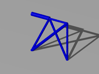
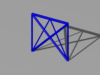
I hope you get the picture of the 2 edges of the polytope in this problem.
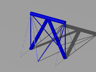
Another interesting point is the fact that we see a 2 dimensional structure in a 3 dimension space. Because the loads are only acting in one plane this is possible. Sure a small perturbation would destroy this behavior. Therefore it is not a practical solution. If you want a practical solution think of robust:
>>> name="2_load_cases_3_dim_robust"
>>> [s,w,lengths] = ttrr.ttrr_robust(dim,nodes,bars,mounting,loads,smax,name=name,sigmamin=sigmamin,sigmamax=sigmamax,density=density,p=0.3,art=0)
And an animation:
$ ttrr_tools.py -xm 320 -ym 240 -f 2_load_cases_3_dim_robust.tar.bz2 --png_pov --apng --mng --gif
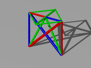
The redundant solution is for a redundancy of 1/3. Every color represent a part of the structure. Every part is allow to drop out. The other parts are able to support the given loads. The interesting point is that the red or blue structure are not connected.
| redundant | robust |
|
|
We can also compare the optimal values (This is the volume of the structures.):
| optimal solution | redundant solution | optimal solution | robust solution |
| simplex | branch and bound | interior point | simplex |
| 0.000875 | 0.001563 | 0.000875 | 0.001154 |