Example: ben-tal_nemirovski_prime_example_1997 ¶

Contents

Example: ben-tal_nemirovski_prime_example_1997

This example shows you how ttrr is used. Some parts are unnecessary, but show the content/meaning of the concerning values or show same features/tools of ttrr. It’s an example file!

This example is also available as batch_ben-tal_nemirovski_prime_example_1997.py.

This example describes the prime example of a truss from: Aharon Ben-Tal and Arkadi Nemirovski. Robust truss topology design via semidefinite programming. SIAM J. Optim., 7(4):991-1016, November 1997. ISSN 1052-6234 (print), 1095-7189 (electronic). http://dx.doi.org/10.1137/S1052623495291951 .

First start python and import necessary modules:

>>> import ttrr,numpy,scipy # we need ttrr and other great packages

design space ¶

To define the design space:

>>> dim = 2 # dimension of the design space
>>> nelx = 3 # number of nodes in x direction
>>> nely = 2 # number of nodes in y direction
>>> kn = nelx*nely # number or total nodes

The definition of the grid:

>>> gx0 = 0.0 # meter
>>> gx1 = 2.0 # meter
>>> gy0 = 0.0 # meter
>>> gy1 = 1.0 # meter

Now we have a design space of nelx*nely=3*2=6 nodes. The design space is a rectangle of the points (x,y) with gx0 <= x <= gx1 and gy0 <= y <= gy1. We need the coordinates of all nodes:

>>> nodes = numpy.array([[ 0.0 , 0.0 ], # node 0 with the coordinates (0.0,0.0) = nodes[0,:]
                          [ 0.0 , 1.0 ], # node 1 with the coordinates (0.0,1.0) = nodes[1,:]
                          [ 1.0 , 0.0 ], # ...
                          [ 1.0 , 1.0 ],
                          [ 2.0 , 0.0 ],
                          [ 2.0 , 1.0 ]],dtype=numpy.float64) # the coordinates are float64 (double)

We need a description of all trusses (from every node to every other one):

>>> bars = numpy.array([[0,2], # truss from node 0 with nodes[0,:] to node 2 with nodes[2,:]
                         [0,1], # truss from node 0 with nodes[0,:] to node 1 with nodes[1,:]
                         [0,3], # ...
                         [0,5],
                         [1,3],
                         [2,4],
                         [1,2],
                         [2,3],
                         [2,5],
                         [3,5],
                         [1,4],
                         [3,4],
                         [4,5]],dtype=numpy.uint16) # the number of nodes are uint16 (16-bit int > 0)

We do not need a truss from 0 to 4 or from 1 to 5, because it is the same as from 0 to 2 and from 2 to 4 or from 1 to 3 and from 3 to 5, respectively.

We can get this from, too (This is handy if you have more than 6 nodes!):

>>> [nodes,bars] = ttrr.barsnodesongrid2d(gx0,gx1,gy0,gy1,nelx,nely)

bearings ¶

We want to fix the node 0 and 1 in every direction:

0 for node 0 in x direction
1 for node 0 in y direction
2 for node 1 in x direction
3 for node 1 in x direction

>>> mounting = numpy.array([0,1,2,3],dtype=numpy.uint16)

The truss from node 0 to node 1 is on both ends fixed. So this truss do not make sense. To reduce the number of design variables we can do it without this truss:

>>> [nodes,bars] = ttrr.barsnodesongrid2d(gx0,gx1,gy0,gy1,nelx,nely,mounting=mounting)
13  potenzielle Staebe gefunden; beruecksichtige 4 Lager
es bleiben 12 Staebe, die nicht nur gelagert sind

load cases ¶

We have only 1 load case, but with “some” forces on different nodes:

>>> loads = scipy.sparse.lil_matrix((dim*kn,1),dtype=numpy.float64)
>>> loads[4,0] = -10000 # force in node 2 in x direction means 4 in the load case 0 with a value of -10000 N; this means a force in -x direction with the magnitude 10000 N in node 2
>>> loads[7,0] = 10000 # force in node 3 in y direction means 7 in the load case 0 with a value of 10000 N; this means a force in y direction with the magnitude 10000 N in node 3
>>> loads[9,0] = -10000 # force in -y direction with the magnitude 10000 N in node 4
>>> loads[10,0] = 10000 # force in x direction with the magnitude 10000 N in node 5

The magnitude of each force is only a scalar factor in the optimization problem. The commanding spot is the proportion of the forces among each other. The same holds for the material parameters.

calculation ¶

We need a few parameters for the calculation:

>>> smax = 1 # the maximum allowed cross section in meter (here: not really a bound)
>>> name = "ben-tal_nemirovski_prime_example" # a name for the output

Some material parameter (The compressive strength sigmamin and the tensile strength sigmamax are only scalar factors in the calculation. The density density is only used to show the mass of the result.):

>>> sigma = 1e8 # Pa = 100 MPa = 100 N / mm^2 (yield strength for aluminium)
>>> sigmamin = - sigma # compressive strength
>>> sigmamax = sigma # tensile strength
>>> density = 2.7e3 # kg / m^3 (density for aluminium)

Now we can calculate the result:

>>> [s,w,lengths] = ttrr.ttrr(dim,nodes,bars,mounting,loads,smax,name=name,sigmamin=sigmamin,sigmamax=sigmamax,density=density)
###### start ttrr ######
tmpdir: /tmp/ttrr_tmp__kA2eC
speichere nach ben-tal_nemirovski_prime_example.tar.bz2
### --- ### --- ### --- ### --- ### --- ### --- ###
starte: ttrr_calculate /tmp/ttrr_tmp__kA2eC
### ttrr ### gestartet ###
lese /tmp/ttrr_tmp__kA2eC/dim.bin
lese /tmp/ttrr_tmp__kA2eC/nodes.bin
lese /tmp/ttrr_tmp__kA2eC/bars.bin
lese /tmp/ttrr_tmp__kA2eC/mounting.bin
lese /tmp/ttrr_tmp__kA2eC/loads.bin
lese /tmp/ttrr_tmp__kA2eC/smax.bin
lese /tmp/ttrr_tmp__kA2eC/info.txt
lese /tmp/ttrr_tmp__kA2eC/redundancy.bin
lese /tmp/ttrr_tmp__kA2eC/opt.bin
lese /tmp/ttrr_tmp__kA2eC/sort.bin
lese /tmp/ttrr_tmp__kA2eC/sigmamin.bin
lese /tmp/ttrr_tmp__kA2eC/sigmamax.bin
lese /tmp/ttrr_tmp__kA2eC/density.bin
lese /tmp/ttrr_tmp__kA2eC/zlb.bin
lese /tmp/ttrr_tmp__kA2eC/zub.bin
ben-tal_nemirovski_prime_example: dim = 2 ; smax = 1.000000e+00 ; redundancy = 0 ; opt = 0 ; sort = 0
sigmamin = -1.000000e+08 ; sigmamax = 1.000000e+08 ; density = 2.700000e+03
6 Knoten ; 12 Staebe ; 4 Lager ; 1 Lastfaelle
calculate geometry matrix and length of bars...geometry matrix (36 non-zero elements) and length of bars calculated
schreibe /tmp/ttrr_tmp__kA2eC/lengths.bin
schreibe /tmp/ttrr_tmp__kA2eC/lengths.txt
schreibe /tmp/ttrr_tmp__kA2eC/C.bin
schreibe /tmp/ttrr_tmp__kA2eC/C.txt
berechne freedofs...freedofs berechnet
schreibe /tmp/ttrr_tmp__kA2eC/freedofs.bin
schreibe /tmp/ttrr_tmp__kA2eC/freedofs.txt
beschraenke Geometriematrix (12x12) auf freie Knoten...Geometriematrix (8x12) auf freie Knoten beschraenkt
schreibe /tmp/ttrr_tmp__kA2eC/C_freedofs.bin
schreibe /tmp/ttrr_tmp__kA2eC/C_freedofs.txt
beschraenke Kraefte (12x1) auf freie Knoten...Kraefte (8x1) auf freie Knoten beschraenkt
schreibe /tmp/ttrr_tmp__kA2eC/loads_freedofs.bin
schreibe /tmp/ttrr_tmp__kA2eC/loads_freedofs.txt
erstelle Optimierungsproblem
berechne Zielfunktion...Zielfunktion berechnet
berechne Gleichungen...8 Gleichungen fuer 24 Unbekannte berechnet (26 Nicht-Null-Elemente)
schreibe /tmp/ttrr_tmp__kA2eC/Aeq.bin
schreibe /tmp/ttrr_tmp__kA2eC/Aeq.txt
schreibe /tmp/ttrr_tmp__kA2eC/beq.bin
schreibe /tmp/ttrr_tmp__kA2eC/beq.txt
berechne Unleichungen...24 Unleichungen fuer 24 Unbekannte berechnet (48 Nicht-Null-Elemente)
schreibe /tmp/ttrr_tmp__kA2eC/A.bin
schreibe /tmp/ttrr_tmp__kA2eC/A.txt
schreibe /tmp/ttrr_tmp__kA2eC/b.bin
schreibe /tmp/ttrr_tmp__kA2eC/b.txt
berechne lb und ub...lb und ub berechnet
schreibe /tmp/ttrr_tmp__kA2eC/lb.bin
schreibe /tmp/ttrr_tmp__kA2eC/lb.txt
schreibe /tmp/ttrr_tmp__kA2eC/ub.bin
schreibe /tmp/ttrr_tmp__kA2eC/ub.txt
A[23,23] = -1.000000e+08
erstelle Gesamtmatrix (32x24) aus 74 Nicht-Null-Elementen...erstellt; lade Gesamtmatrix...Gesamtmatrix geladen
Writing problem data to `/tmp/ttrr_tmp__kA2eC/ben-tal_nemirovski_prime_example.glpk.gz'...
69 lines were written
Writing problem data to `/tmp/ttrr_tmp__kA2eC/ben-tal_nemirovski_prime_example.prob.gz'...
141 lines were written
berechne...
opt == 0: glp_simplex
GLPK Simplex Optimizer, v4.45
32 rows, 24 columns, 74 non-zeros
Preprocessing...
32 rows, 24 columns, 74 non-zeros
Scaling...
 A: min|aij| =  4.472e-01  max|aij| =  1.000e+08  ratio =  2.236e+08
GM: min|aij| =  8.286e-01  max|aij| =  1.207e+00  ratio =  1.456e+00
EQ: min|aij| =  7.071e-01  max|aij| =  1.000e+00  ratio =  1.414e+00
Constructing initial basis...
Size of triangular part = 32
      0: obj =   0.000000000e+00  infeas =  1.740e+09 (0)
*    26: obj =   1.300000000e-03  infeas =  3.150e-12 (0)
*    29: obj =   8.000000000e-04  infeas =  8.078e-28 (0)
OPTIMAL SOLUTION FOUND
Writing basic solution to `/tmp/ttrr_tmp__kA2eC/ben-tal_nemirovski_prime_example.out.gz'...
Writing basic solution to `/tmp/ttrr_tmp__kA2eC/ben-tal_nemirovski_prime_example.sol.gz'...
58 lines were written
Zielfunktionswert: 0.000800
Gesamtvolumen: 0.000800
Gesamtgewicht: 2.160000
schreibe /tmp/ttrr_tmp__kA2eC/w.bin
schreibe /tmp/ttrr_tmp__kA2eC/w.txt
schreibe /tmp/ttrr_tmp__kA2eC/s.bin
schreibe /tmp/ttrr_tmp__kA2eC/s.txt
schreibe /tmp/ttrr_tmp__kA2eC/objectivefunctionvalue.bin
schreibe /tmp/ttrr_tmp__kA2eC/objectivefunctionvalue.txt
gebe Speicher wieder frei
### ttrr ### beendet ###
### --- ### --- ### --- ### --- ### --- ### --- ###
speichere nach ben-tal_nemirovski_prime_example.tar.bz2
###### end ttrr ######

As in “Aharon Ben-Tal and Arkadi Nemirovski. Robust truss topology design via semidefinite programming. SIAM J. Optim., 7(4):991-1016, November 1997. ISSN 1052-6234 (print), 1095-7189 (electronic). http://dx.doi.org/10.1137/S1052623495291951 .” we can get a robust solution; but here with a linear program as described in “Mohr, Daniel P. ; Stein, Ina ; Matzies, Thomas ; Knapek, Christina A.: Robust Topology Optimization of Truss with regard to Volume. In: arXiv - Mathematics, Optimization and Control (2012). http://arxiv.org/abs/1109.3782” (This time the output is omitted.):

>>> name = "ben-tal_nemirovski_prime_example_robust" # a name for the output
>>> [s,w,lengths] = ttrr.ttrr_robust(dim,nodes,bars,mounting,loads,smax,name=name,sigmamin=sigmamin,sigmamax=sigmamax,density=density,p=0.1,art=0)

More explicitly we can calculate (or even define) the perturbed forces:

>>> forces_disturbed = ttrr.compute_disturbed_forces(loads,dim,0.1,art=0)
###### compute_disturbed_forces
(kkn,nl) = (12,1); Knotenzahl: 6; Dimension: 2
###### compute_disturbed_forces
(kkn,nl) = (12,1); Knotenzahl: 6; Dimension: 2
######
max_force_undisturbed = 20000.000000
max_force_disturbed = 20784.609691
skaliere Kraefte
max_force_disturbed = 20000.000000
######

And do the computation with these (The output is omitted.):

>>> [s,w,lengths] = ttrr.ttrr(dim,nodes,bars,mounting,forces_disturbed,smax,name=name,sigmamin=sigmamin,sigmamax=sigmamax,density=density)

For the same problem we can calculate a (1/2)-redundant solution as described in “Mohr, Daniel P. ; Stein, Ina ; Matzies, Thomas ; Knapek, Christina A.: Redundant robust topology optimization of truss. In: Optimization and Engineering (2013), 1-28. http://dx.doi.org/10.1007/s11081-013-9241-7” and in “Mohr, Daniel P.: Redundante Topologieoptimierung. Neubiberg, Universitaet der Bundeswehr Muenchen, Fakultaet fuer Luft- und Raumfahrttechnik, Diss., Dezember 2011. http://nbn-resolving.de/urn/resolver.pl?urn=urn:nbn:de:bvb:706-2664”:

>>> name = "ben-tal_nemirovski_prime_example_redundant" # a name for the output
>>> [s,w,lengths] = ttrr.ttrr_redundant(dim,nodes,bars,mounting,loads,smax,name=name,sigmamin=sigmamin,sigmamax=sigmamax,density=density,redundancy=2,opt=3)

visualization ¶

To get pictures, we can use ttrr_tools.py on the command line:

$ ttrr_tools.py --png_gnuplot -f ben-tal_nemirovski_prime_example.tar.bz2 ben-tal_nemirovski_prime_example_robust.tar.bz2 ben-tal_nemirovski_prime_example_redundant.tar.bz2

Or for short:

$ ttrr_tools.py --png_gnuplot -f ben-tal_nemirovski_prime_example*.tar.bz2

Now we get the example pictures:

optimal solution	robust solution	redundant solution

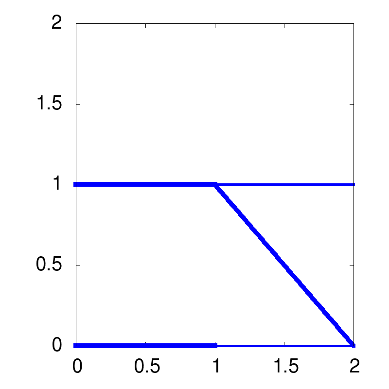
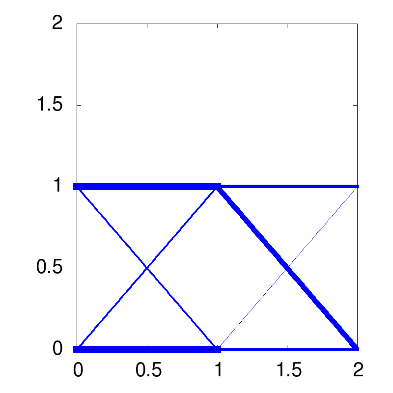
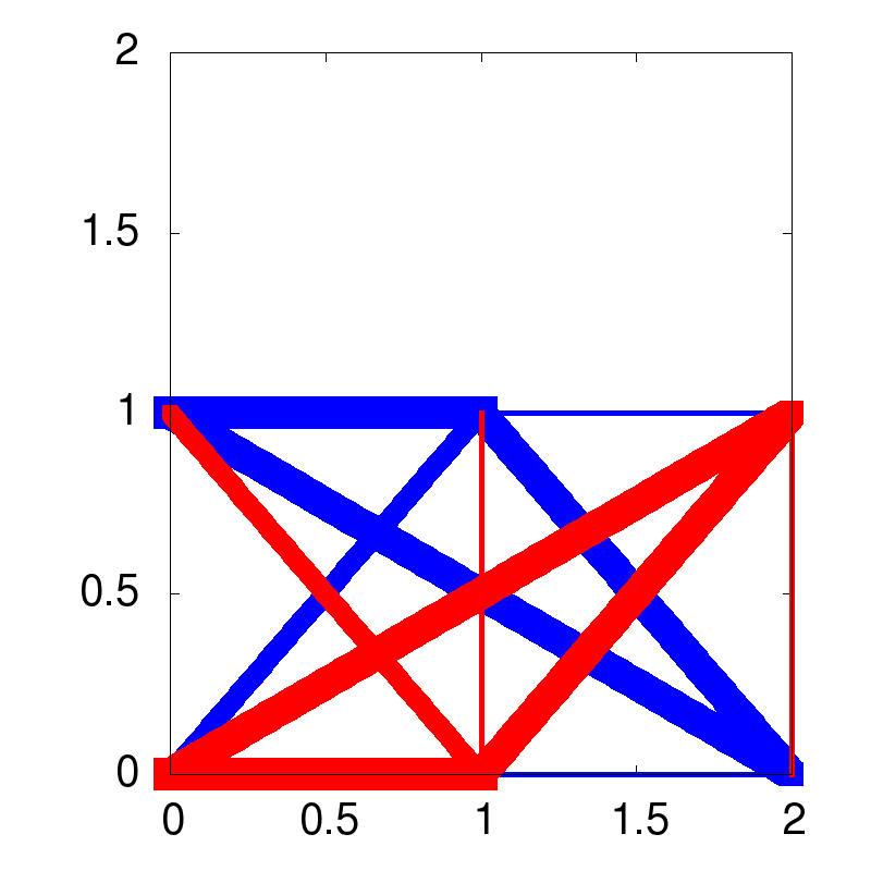
I think these pictures are the best way for our human being to understand the topologies. Keep in mind that the topology is not the sizing of parts of the structure. But the calculation needs the sizing values to benchmark the topology. So it is impossible to get a topology of a structure without the sizing values.

conclusion ¶

The degree of freedom for this problem is very small. This means: The set of admissible solutions is small. So the optimization routine has only a small choice. The consequence is that in particular the result of the redundant solution is poor. But this file shows the functionality of ttrr and also the basic concept of robustness and redundancy. I hope you get the point.

Example: ben-tal_nemirovski_prime_example_1997 ¶

design space ¶

bearings ¶

load cases ¶

calculation ¶

visualization ¶

conclusion ¶

Table Of Contents

Previous topic

Next topic

This Page

Navigation

Previous topic

Next topic

This Page

Quick search

Navigation